412 lines
17 KiB
Markdown
412 lines
17 KiB
Markdown
# 25 | 如何用法线贴图模拟真实物体表面
|
||
|
||
你好,我是月影。
|
||
|
||
上节课,我们讲了光照的Phong反射模型,并使用它给几何体添加了光照效果。不过,我们使用的几何体表面都是平整的,没有凹凸感。而真实世界中,大部分物体的表面都是凹凸不平的,这肯定会影响光照的反射效果。
|
||
|
||
因此,只有处理好物体凹凸表面的光照效果,我们才能更加真实地模拟物体表面。在图形学中就有一种对应的技术,叫做**法线贴图**。今天,我们就一起来学习一下。
|
||
|
||
## 如何使用法线贴图给几何体表面增加凹凸效果?
|
||
|
||
那什么是法线贴图?我们直接通过一个例子来理解。
|
||
|
||
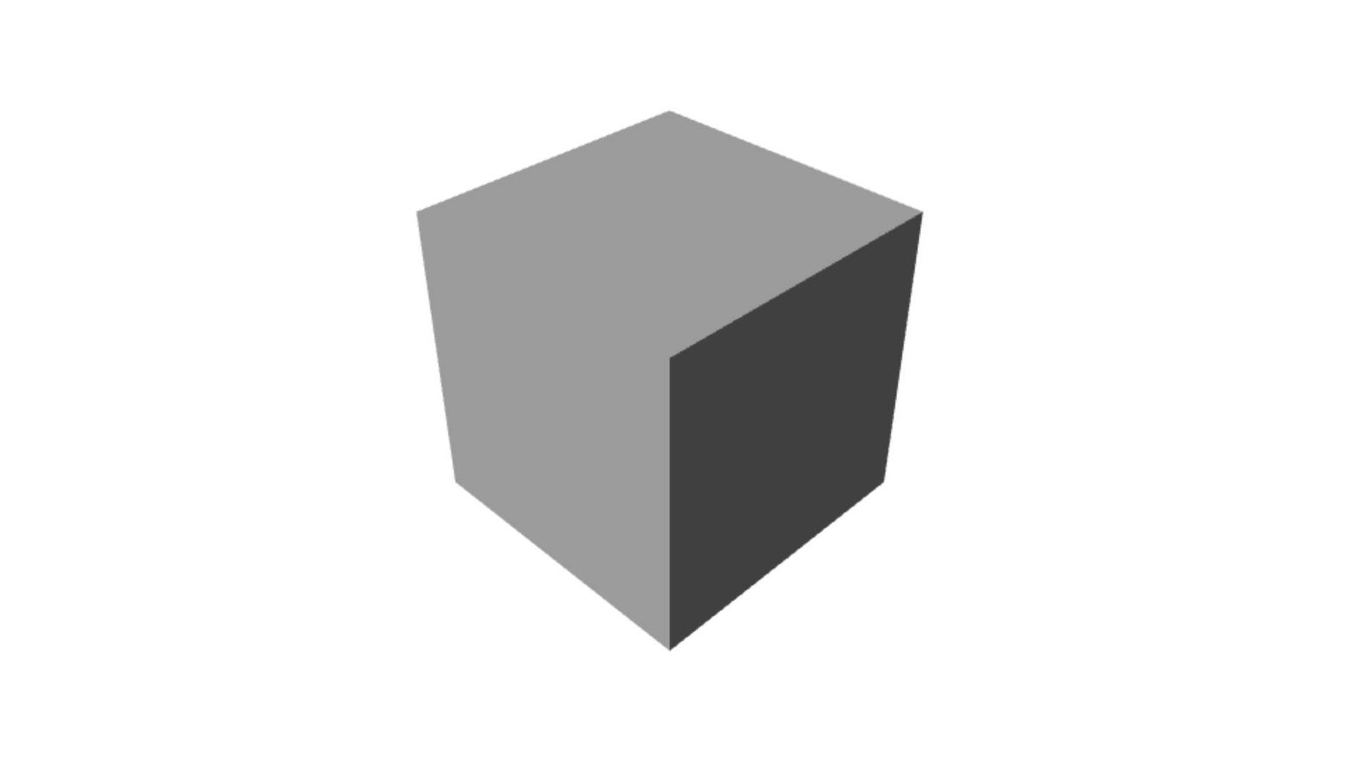
首先,我们用Phong反射模型绘制一个灰色的立方体,并给它添加两道平行光。具体的代码和效果如下:
|
||
|
||
```
|
||
import {Phong, Material, vertex as v, fragment as f} from '../common/lib/phong.js';
|
||
|
||
const scene = new Transform();
|
||
|
||
const phong = new Phong();
|
||
phong.addLight({
|
||
direction: [0, -3, -3],
|
||
});
|
||
phong.addLight({
|
||
direction: [0, 3, 3],
|
||
});
|
||
const matrial = new Material(new Color('#808080'));
|
||
|
||
const program = new Program(gl, {
|
||
vertex: v,
|
||
fragment: f,
|
||
uniforms: {
|
||
...phong.uniforms,
|
||
...matrial.uniforms,
|
||
},
|
||
});
|
||
|
||
const geometry = new Box(gl);
|
||
const cube = new Mesh(gl, {geometry, program});
|
||
cube.setParent(scene);
|
||
cube.rotation.x = -Math.PI / 2;
|
||
|
||
```
|
||
|
||
|
||
|
||
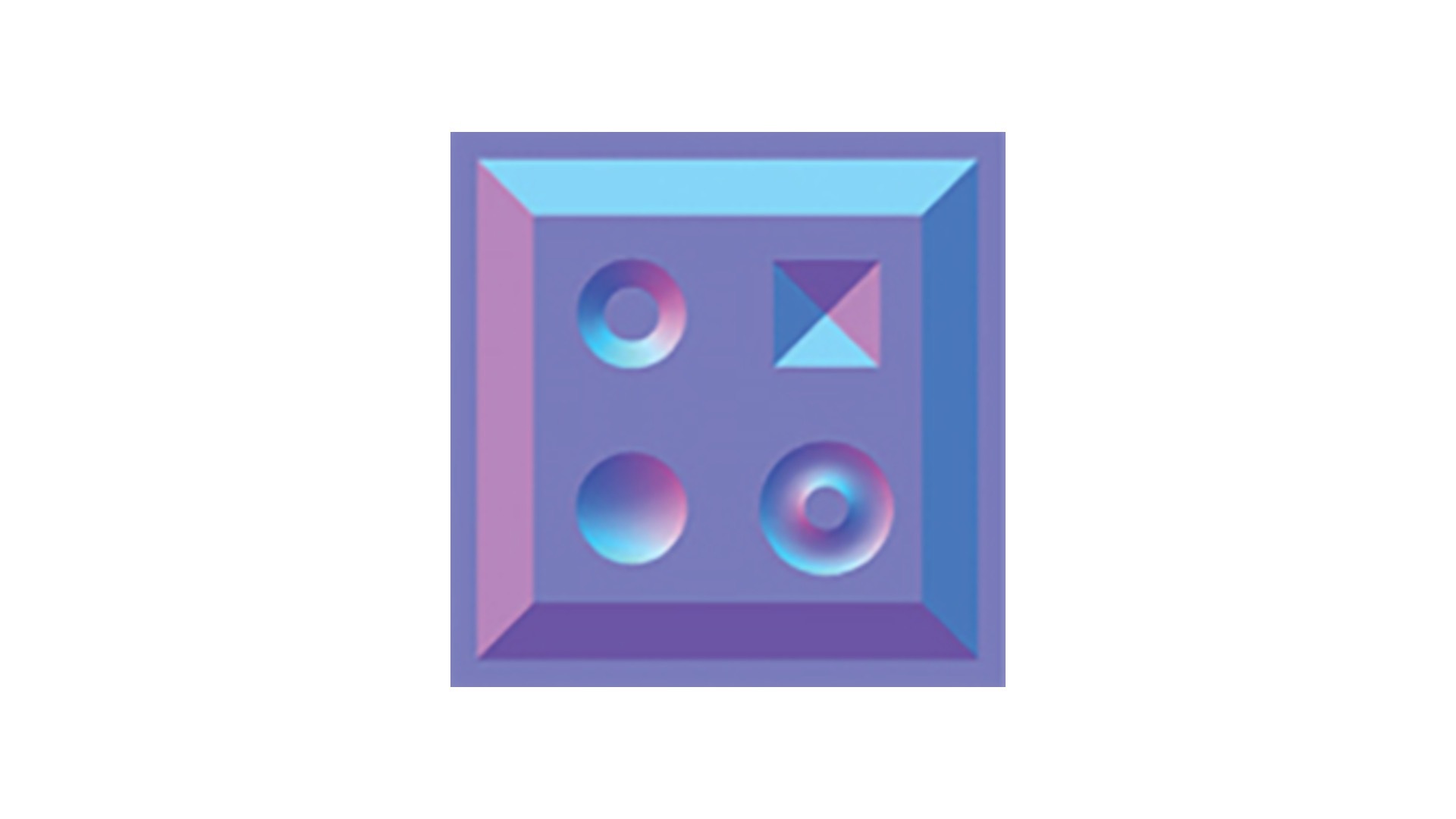
现在这个立方体的表面是光滑的,如果我们想在立方体的表面贴上凹凸的花纹。我们可以加载一张**法线纹理**,这是一张偏蓝色调的纹理图片。
|
||
|
||
|
||
|
||
```
|
||
const normalMap = await loadTexture('../assets/normal_map.png');
|
||
|
||
```
|
||
|
||
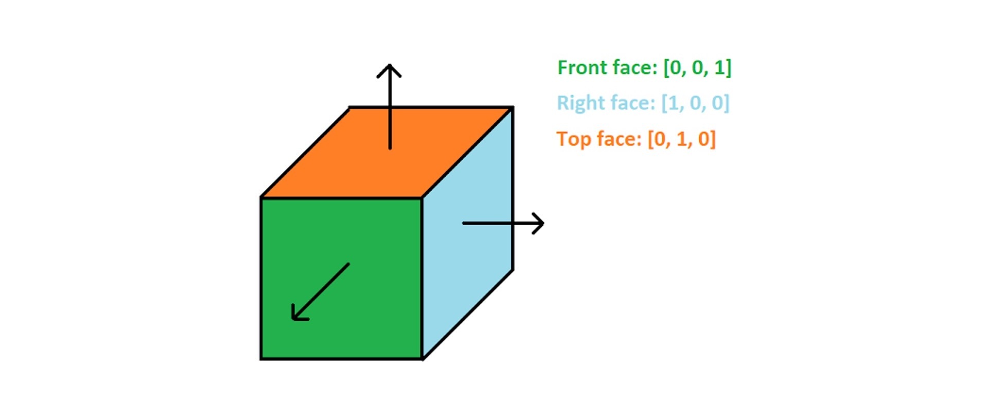
为什么这张纹理图片是偏蓝色调的呢?实际上,这张纹理图片保存的是几何体表面的每个像素的法向量数据。我们知道,正常情况下,光滑立方体每个面的法向量是固定的,如下图所示:
|
||
|
||
[](http://www.mbsoftworks.sk/tutorials/opengl4/014-normals-diffuse-lighting/)
|
||
|
||
但如果表面有凹凸的花纹,那不同位置的法向量就会发生变化。在**切线空间**中,因为法线都偏向于z轴,也就是法向量偏向于(0,0,1),所以转换成的法线纹理就偏向于蓝色。如果我们根据花纹将每个点的法向量都保存下来,就会得到上面那张法线纹理的图片。
|
||
|
||
### 如何理解切线空间?
|
||
|
||
我刚才提到了一个词,切线空间,那什么是切线空间呢?切线空间(Tangent Space)是一个特殊的坐标系,它是由几何体顶点所在平面的uv坐标和法线构成的。
|
||
|
||
[](https://math.stackexchange.com/questions/342211/difference-between-tangent-space-and-tangent-plane)
|
||
|
||
切线空间的三个轴,一般用 T (Tangent)、B (Bitangent)、N (Normal) 三个字母表示,所以切线空间也被称为TBN空间。其中T表示切线、B表示副切线、N表示法线。
|
||
|
||
对于大部分三维几何体来说,因为每个点的法线不同,所以它们各自的切线空间也不同。
|
||
|
||
接下来,我们来具体说说,切线空间中的TBN是怎么计算的。
|
||
|
||
首先,我们来回忆一下,怎么计算几何体三角形网格的法向量。假设一个三角形网格有三个点v1、v2、v3,我们把边v1v2记为e1,边v1v3记为e2,那三角形的法向量就是e1和e2的叉积表示的归一化向量。用JavaScript代码实现就是下面这样:
|
||
|
||
```
|
||
function getNormal(v1, v2, v3) {
|
||
const e1 = Vec3.sub(v2, v1);
|
||
const e2 = Vec3.sub(v3, v1);
|
||
const normal = Vec3.cross(e1, e1).normalize();
|
||
return normal;
|
||
}
|
||
|
||
```
|
||
|
||
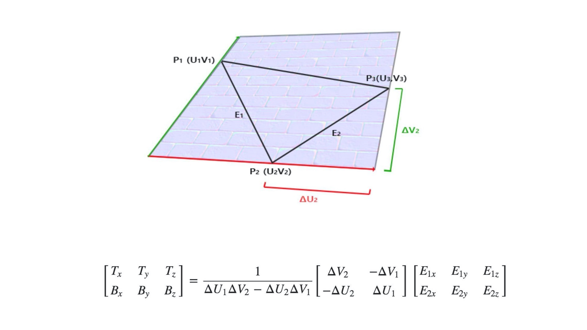
而计算切线和副切线,要比计算法线复杂得多,不过,因为[数学推导过程](https://learnopengl.com/Advanced-Lighting/Normal-Mapping)比较复杂,我们只要记住结论就可以了。
|
||
|
||
|
||
|
||
如上图和公式,我们就可以通过UV坐标和点P1、P2、P3的坐标求出对应的T和B坐标了,对应的JavaScript函数如下:
|
||
|
||
```
|
||
function createTB(geometry) {
|
||
const {position, index, uv} = geometry.attributes;
|
||
if(!uv) throw new Error('NO uv.');
|
||
function getTBNTriangle(p1, p2, p3, uv1, uv2, uv3) {
|
||
const edge1 = new Vec3().sub(p2, p1);
|
||
const edge2 = new Vec3().sub(p3, p1);
|
||
const deltaUV1 = new Vec2().sub(uv2, uv1);
|
||
const deltaUV2 = new Vec2().sub(uv3, uv1);
|
||
|
||
const tang = new Vec3();
|
||
const bitang = new Vec3();
|
||
|
||
const f = 1.0 / (deltaUV1.x * deltaUV2.y - deltaUV2.x * deltaUV1.y);
|
||
|
||
tang.x = f * (deltaUV2.y * edge1.x - deltaUV1.y * edge2.x);
|
||
tang.y = f * (deltaUV2.y * edge1.y - deltaUV1.y * edge2.y);
|
||
tang.z = f * (deltaUV2.y * edge1.z - deltaUV1.y * edge2.z);
|
||
|
||
tang.normalize();
|
||
|
||
bitang.x = f * (-deltaUV2.x * edge1.x + deltaUV1.x * edge2.x);
|
||
bitang.y = f * (-deltaUV2.x * edge1.y + deltaUV1.x * edge2.y);
|
||
bitang.z = f * (-deltaUV2.x * edge1.z + deltaUV1.x * edge2.z);
|
||
|
||
bitang.normalize();
|
||
|
||
return {tang, bitang};
|
||
}
|
||
|
||
const size = position.size;
|
||
if(size < 3) throw new Error('Error dimension.');
|
||
|
||
const len = position.data.length / size;
|
||
const tang = new Float32Array(len * 3);
|
||
const bitang = new Float32Array(len * 3);
|
||
|
||
for(let i = 0; i < index.data.length; i += 3) {
|
||
const i1 = index.data[i];
|
||
const i2 = index.data[i + 1];
|
||
const i3 = index.data[i + 2];
|
||
|
||
const p1 = [position.data[i1 * size], position.data[i1 * size + 1], position.data[i1 * size + 2]];
|
||
const p2 = [position.data[i2 * size], position.data[i2 * size + 1], position.data[i2 * size + 2]];
|
||
const p3 = [position.data[i3 * size], position.data[i3 * size + 1], position.data[i3 * size + 2]];
|
||
|
||
const u1 = [uv.data[i1 * 2], uv.data[i1 * 2 + 1]];
|
||
const u2 = [uv.data[i2 * 2], uv.data[i2 * 2 + 1]];
|
||
const u3 = [uv.data[i3 * 2], uv.data[i3 * 2 + 1]];
|
||
|
||
const {tang: t, bitang: b} = getTBNTriangle(p1, p2, p3, u1, u2, u3);
|
||
tang.set(t, i1 * 3);
|
||
tang.set(t, i2 * 3);
|
||
tang.set(t, i3 * 3);
|
||
bitang.set(b, i1 * 3);
|
||
bitang.set(b, i2 * 3);
|
||
bitang.set(b, i3 * 3);
|
||
}
|
||
geometry.addAttribute('tang', {data: tang, size: 3});
|
||
geometry.addAttribute('bitang', {data: bitang, size: 3});
|
||
return geometry;
|
||
}
|
||
|
||
|
||
```
|
||
|
||
虽然上面这段代码比较长,但并不复杂。具体的思路就是按照我给出的公式,先进行向量计算,然后将tang和bitang的值添加到geometry对象中去。
|
||
|
||
### 构建TBN矩阵来计算法向量
|
||
|
||
有了tang和bitang之后,我们就可以构建TBN矩阵来计算法线了。这里的TBN矩阵的作用,就是将法线贴图里面读取的法向量数据,转换为对应的切线空间中实际的法向量。这里的切线空间,实际上对应着我们观察者(相机)位置的坐标系。
|
||
|
||
接下来,我们对应顶点着色器和片元着色器来说说,怎么构建TBN矩阵得出法线方向。
|
||
|
||
先看顶点着色器,我们增加了tang和bitang这两个属性。注意,这里我们用了webgl2.0的写法,因为WebGL2.0对应OpenGL ES3.0,所以这段代码和我们之前看到的着色器代码略有不同。
|
||
|
||
首先它的第一行声明 #version 300 es 表示这段代码是OpenGL ES3.0的,然后我们用in和out对应变量的输入和输出,来取代WebGL2.0的attribute和varying,其他的地方基本和WebGL1.0一样。因为OGL默认支持WebGL2.0,所以在后续例子中你还会看到更多OpenGL ES3.0的着色器写法,不过因为两个版本差别不大,也不会妨碍我们理解代码。
|
||
|
||
```
|
||
#version 300 es
|
||
precision highp float;
|
||
|
||
in vec3 position;
|
||
in vec3 normal;
|
||
in vec2 uv;
|
||
in vec3 tang;
|
||
in vec3 bitang;
|
||
|
||
uniform mat4 modelMatrix;
|
||
uniform mat4 modelViewMatrix;
|
||
uniform mat4 viewMatrix;
|
||
uniform mat4 projectionMatrix;
|
||
uniform mat3 normalMatrix;
|
||
uniform vec3 cameraPosition;
|
||
|
||
out vec3 vNormal;
|
||
out vec3 vPos;
|
||
out vec2 vUv;
|
||
out vec3 vCameraPos;
|
||
out mat3 vTBN;
|
||
|
||
void main() {
|
||
vec4 pos = modelViewMatrix * vec4(position, 1.0);
|
||
vPos = pos.xyz;
|
||
vUv = uv;
|
||
vCameraPos = (viewMatrix * vec4(cameraPosition, 1.0)).xyz;
|
||
vNormal = normalize(normalMatrix * normal);
|
||
|
||
vec3 N = vNormal;
|
||
vec3 T = normalize(normalMatrix * tang);
|
||
vec3 B = normalize(normalMatrix * bitang);
|
||
|
||
vTBN = mat3(T, B, N);
|
||
|
||
gl_Position = projectionMatrix * pos;
|
||
}
|
||
|
||
|
||
```
|
||
|
||
接着来看代码,我们通过normal、tang和bitang建立TBN矩阵。注意,因为normal、tang和bitang都需要换到世界坐标中,所以我们要记得将它们左乘法向量矩阵normalMatrix,然后我们构建TBN矩阵(vTBN=mat(T,B,N)),将它传给片元着色器。
|
||
|
||
下面,我们接着来看片元着色器。
|
||
|
||
```
|
||
#version 300 es
|
||
precision highp float;
|
||
|
||
#define MAX_LIGHT_COUNT 16
|
||
uniform mat4 viewMatrix;
|
||
|
||
uniform vec3 ambientLight;
|
||
uniform vec3 directionalLightDirection[MAX_LIGHT_COUNT];
|
||
uniform vec3 directionalLightColor[MAX_LIGHT_COUNT];
|
||
uniform vec3 pointLightColor[MAX_LIGHT_COUNT];
|
||
uniform vec3 pointLightPosition[MAX_LIGHT_COUNT];
|
||
uniform vec3 pointLightDecay[MAX_LIGHT_COUNT];
|
||
uniform vec3 spotLightColor[MAX_LIGHT_COUNT];
|
||
uniform vec3 spotLightDirection[MAX_LIGHT_COUNT];
|
||
uniform vec3 spotLightPosition[MAX_LIGHT_COUNT];
|
||
uniform vec3 spotLightDecay[MAX_LIGHT_COUNT];
|
||
uniform float spotLightAngle[MAX_LIGHT_COUNT];
|
||
|
||
uniform vec3 materialReflection;
|
||
uniform float shininess;
|
||
uniform float specularFactor;
|
||
|
||
uniform sampler2D tNormal;
|
||
|
||
in vec3 vNormal;
|
||
in vec3 vPos;
|
||
in vec2 vUv;
|
||
in vec3 vCameraPos;
|
||
in mat3 vTBN;
|
||
|
||
out vec4 FragColor;
|
||
|
||
float getSpecular(vec3 dir, vec3 normal, vec3 eye) {
|
||
vec3 reflectionLight = reflect(-dir, normal);
|
||
float eyeCos = max(dot(eye, reflectionLight), 0.0);
|
||
return specularFactor * pow(eyeCos, shininess);
|
||
}
|
||
|
||
vec4 phongReflection(vec3 pos, vec3 normal, vec3 eye) {
|
||
float specular = 0.0;
|
||
vec3 diffuse = vec3(0);
|
||
|
||
// 处理平行光
|
||
for(int i = 0; i < MAX_LIGHT_COUNT; i++) {
|
||
vec3 dir = directionalLightDirection[i];
|
||
if(dir.x == 0.0 && dir.y == 0.0 && dir.z == 0.0) continue;
|
||
vec4 d = viewMatrix * vec4(dir, 0.0);
|
||
dir = normalize(-d.xyz);
|
||
float cos = max(dot(dir, normal), 0.0);
|
||
diffuse += cos * directionalLightColor[i];
|
||
specular += getSpecular(dir, normal, eye);
|
||
}
|
||
|
||
// 处理点光源
|
||
for(int i = 0; i < MAX_LIGHT_COUNT; i++) {
|
||
vec3 decay = pointLightDecay[i];
|
||
if(decay.x == 0.0 && decay.y == 0.0 && decay.z == 0.0) continue;
|
||
vec3 dir = (viewMatrix * vec4(pointLightPosition[i], 1.0)).xyz - pos;
|
||
float dis = length(dir);
|
||
dir = normalize(dir);
|
||
float cos = max(dot(dir, normal), 0.0);
|
||
float d = min(1.0, 1.0 / (decay.x * pow(dis, 2.0) + decay.y * dis + decay.z));
|
||
diffuse += d * cos * pointLightColor[i];
|
||
specular += getSpecular(dir, normal, eye);
|
||
}
|
||
|
||
// 处理聚光灯
|
||
for(int i = 0; i < MAX_LIGHT_COUNT; i++) {
|
||
vec3 decay = spotLightDecay[i];
|
||
if(decay.x == 0.0 && decay.y == 0.0 && decay.z == 0.0) continue;
|
||
|
||
vec3 dir = (viewMatrix * vec4(spotLightPosition[i], 1.0)).xyz - pos;
|
||
float dis = length(dir);
|
||
dir = normalize(dir);
|
||
|
||
// 聚光灯的朝向
|
||
vec3 spotDir = (viewMatrix * vec4(spotLightDirection[i], 0.0)).xyz;
|
||
// 通过余弦值判断夹角范围
|
||
float ang = cos(spotLightAngle[i]);
|
||
float r = step(ang, dot(dir, normalize(-spotDir)));
|
||
|
||
float cos = max(dot(dir, normal), 0.0);
|
||
float d = min(1.0, 1.0 / (decay.x * pow(dis, 2.0) + decay.y * dis + decay.z));
|
||
diffuse += r * d * cos * spotLightColor[i];
|
||
specular += r * getSpecular(dir, normal, eye);
|
||
}
|
||
|
||
return vec4(diffuse, specular);
|
||
}
|
||
|
||
vec3 getNormal() {
|
||
vec3 n = texture(tNormal, vUv).rgb * 2.0 - 1.0;
|
||
return normalize(vTBN * n);
|
||
}
|
||
|
||
void main() {
|
||
vec3 eyeDirection = normalize(vCameraPos - vPos);
|
||
vec3 normal = getNormal();
|
||
vec4 phong = phongReflection(vPos, normal, eyeDirection);
|
||
|
||
// 合成颜色
|
||
FragColor.rgb = phong.w + (phong.xyz + ambientLight) * materialReflection;
|
||
FragColor.a = 1.0;
|
||
}
|
||
|
||
|
||
```
|
||
|
||
片元着色器代码虽然也很长,但也并不复杂。因为其中的Phong反射模型,我们已经比较熟悉了。剩下的部分,我们重点理解,怎么从法线纹理中提取数据和TBN矩阵,来计算对应的法线就行了。具体的计算方法就是把法线纹理贴图中提取的数据转换到\[-1,1\]区间,然后左乘TBN矩阵并归一化。
|
||
|
||
然后,我们将经过处理之后的法向量传给phongReflection计算光照,就得到了法线贴图后的结果,效果如下图:
|
||
|
||
|
||
|
||
到这里我们就实现了完整的法线贴图。法线贴图就是根据法线纹理中保存的法向量数据以及TBN矩阵,将实际的法线计算出来,然后用实际的法线来计算光照的反射。具体点来说,要实现法线贴图,我们需要通过顶点数据计算几何体的切线和副切线,然后得到TBN矩阵,用TBN矩阵和法线纹理数据来计算法向量,从而完成法线贴图。
|
||
|
||
### 使用偏导数来实现法线贴图
|
||
|
||
但是,构建TBN矩阵求法向量的方法还是有点麻烦。事实上,还有一种更巧妙的方法,不需要用顶点数据计算几何体的切线和副切线,而是直接用坐标插值和法线纹理来计算。
|
||
|
||
```
|
||
vec3 getNormal() {
|
||
vec3 pos_dx = dFdx(vPos.xyz);
|
||
vec3 pos_dy = dFdy(vPos.xyz);
|
||
vec2 tex_dx = dFdx(vUv);
|
||
vec2 tex_dy = dFdy(vUv);
|
||
|
||
vec3 t = normalize(pos_dx * tex_dy.t - pos_dy * tex_dx.t);
|
||
vec3 b = normalize(-pos_dx * tex_dy.s + pos_dy * tex_dx.s);
|
||
mat3 tbn = mat3(t, b, normalize(vNormal));
|
||
|
||
vec3 n = texture(tNormal, vUv).rgb * 2.0 - 1.0;
|
||
return normalize(tbn * n);
|
||
}
|
||
|
||
```
|
||
|
||
如上面代码所示,dFdx、dFdy是GLSL内置函数,可以求插值的属性在x、y轴上的偏导数。那我们为什么要求偏导数呢?**偏导数**其实就代表插值的属性向量在x、y轴上的变化率,或者说曲面的切线。然后,我们再将顶点坐标曲面切线与uv坐标的切线求叉积,就能得到垂直于两条切线的法线。
|
||
|
||
那我们在x、y两个方向上求出的两条法线,就对应TBN空间的切线tang和副切线bitang。然后,我们使用偏导数构建TBN矩阵,同样也是把TBN矩阵左乘从法线纹理中提取出的值,就可以计算出对应的法向量了。
|
||
|
||
这样做的好处是,我们不需要预先计算几何体的tang和bitang了。不过在片元着色器中计算偏导数也有一定的性能开销,所以各有利弊,我们可以根据不同情况选择不同的方案。
|
||
|
||
## 法线贴图的应用
|
||
|
||
法线贴图的两种实现方式,我们都学会了。那法线贴图除了给几何体表面增加花纹以外,还可以用来增强物体细节,让物体看起来更加真实。比如说,在实现一个石块被变化的光源照亮效果的时候,我们就可以运用法线贴图技术,让石块的表面纹路细节显得非常的逼真。我把对应的片元着色器核心代码放在了下面,你可以利用今天学到的知识自己来实现一下。
|
||
|
||
|
||
|
||
```
|
||
uniform float uTime;
|
||
|
||
void main() {
|
||
vec3 eyeDirection = normalize(vCameraPos - vPos);
|
||
vec3 normal = getNormal();
|
||
vec4 phong = phongReflection(vPos, normal, eyeDirection);
|
||
// vec4 phong = phongReflection(vPos, vNormal, eyeDirection);
|
||
|
||
vec3 tex = texture(tMap, vUv).rgb;
|
||
vec3 light = normalize(vec3(sin(uTime), 1.0, cos(uTime)));
|
||
float shading = dot(normal, light) * 0.5;
|
||
|
||
FragColor.rgb = tex + shading;
|
||
FragColor.a = 1.0;
|
||
}
|
||
|
||
```
|
||
|
||
## 要点总结
|
||
|
||
这节课,我们详细说了法线贴图这个技术。法线贴图是一种经典的图形学技术,可以用来给物体表面增加细节,让我们实现的效果更逼真。
|
||
|
||
具体来说,法线贴图是用一张图片来存储表面的法线数据。这张图片叫做法线纹理,它上面的每个像素对应一个坐标点的法线数据。
|
||
|
||
要想使用法线纹理的数据,我们还需要构建TBN矩阵。这个矩阵通过向量、矩阵乘法将法线数据转换到世界坐标中。
|
||
|
||
构建TBN矩阵我们有两个方法,一个是根据几何体顶点数据来计算切线(Tangent)、副切线(Bitangent),然后结合法向量一起构建TBN矩阵。另一个方法是使用偏导数来计算,这样我们就不用预先在顶点中计算Tangent和Bitangent了。两种方法各有利弊,我们可以根据实际情况来合理选择。
|
||
|
||
## 小试牛刀
|
||
|
||
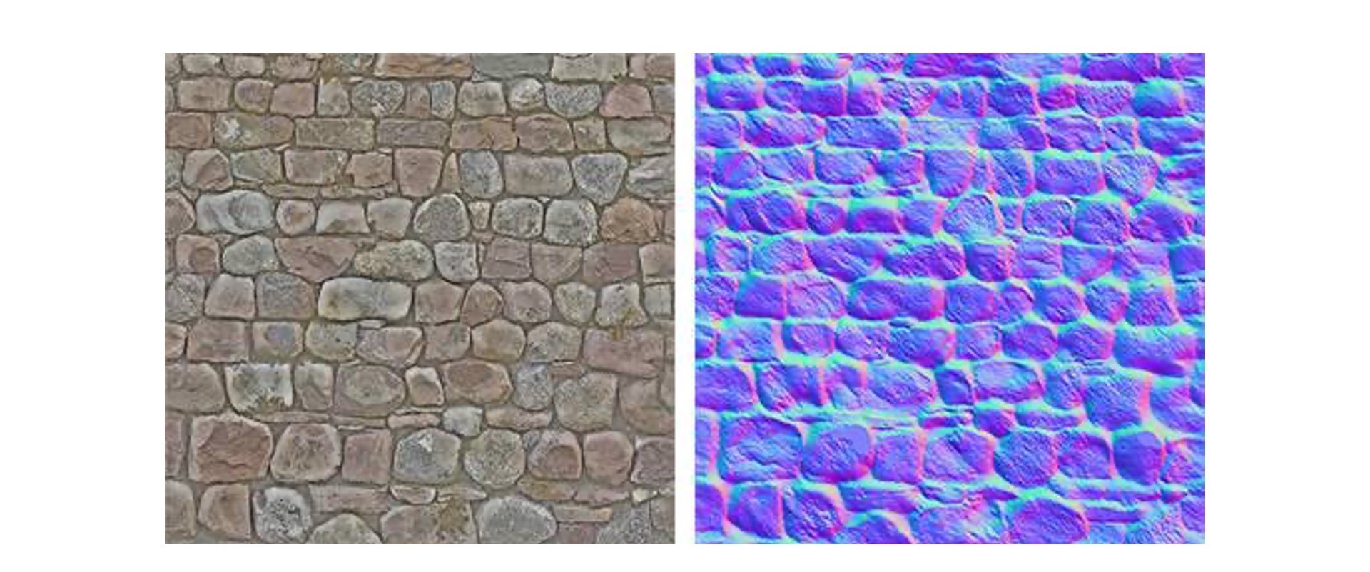
这里,我给出了两张图片,一张是纹理图片,一张是法线纹理,你能用它们分别来绘制一面墙,并且引入Phong反射模型,来实现光照效果吗?你还可以思考一下,应用法线贴图和不应用法线贴图绘制出来的墙,有什么差别?
|
||
|
||
|
||
|
||
欢迎在留言区和我讨论,分享你的答案和思考,也欢迎你把这节课分享给你的朋友,我们下节课再见!
|
||
|
||
* * *
|
||
|
||
## 源码
|
||
|
||
课程中完整示例代码见[GitHub仓库](https://github.com/akira-cn/graphics/tree/master/normal-maps)
|
||
|
||
## 推荐阅读
|
||
|
||
[Normal mapping](https://learnopengl.com/Advanced-Lighting/Normal-Mapping)
|
||
|